TL;DR

Web scraping can be an incredibly useful tool to obtain a dataset from the internet. In this analysis, we scrape some review data from Amazon before performing some basic text analysis on this data.

Introduction

Web scraping is a method for extracting data from web pages which can then be used in an analysis. It can be an incredibly useful tool to collect data to compliment analysis being conducted on another dataset or as a separate analysis on its own. Luckily, R offers a package which allows us to perform web scraping called rvest.

As a main interest area of research for me is digital health technologies, I have read many papers that examine users experiences with such devices. These papers come with a number of limitations. Firstly, the amount of time taken to planthe study, collect and analyse the results and then have them published the consumer market has moved on (usually by at least one generation) making the findings less useful. On top of this, such studies come with associated costs. This has led me to think, is there a better way to collect users experiences of digital health technologies without conducting a full academic study? This led me to thinking about web-scraping Amazon reviews.

Amazon reviews provide a large collection of users self-reported experience with different digital health technologies. As rvest provides a simple means to web scrape such information within R, this analysis will focus on highlighting how such data can be collected and analysed.

The idea for this analysis came from Martin Chan’s blog post on this subject. The concept for the web scraping code has been adapted from this blog along with the excellent explanations provided.

Web scraping

The function below (scrape_amazon) allows us to scrape the information from Amazon reviews. This function takes two inputs: the amazon_url which is the the link to the first page of reviews for the given item, and the page number we want to scrape the reviews from. We then extract 5 key elements from the Amazon reviews: their title, the review text, the number of stars given in the review and the date the review was published. These lists are then combined into a dataframe.

scrape_amazon <- function(amazon_url, page_num){
  
  url_reviews <- paste(amazon_url,page_num, sep = "")
  
  doc <- read_html(url_reviews) # Assign results to `doc`
  
  # Review Title
  doc %>% 
    html_nodes("[class='a-size-base a-link-normal review-title a-color-base review-title-content a-text-bold']") %>%
    html_text() -> review_title
  
  # Review Text
  doc %>% 
    html_nodes("[class='a-size-base review-text review-text-content']") %>%
    html_text() -> review_text
  
  # Number of stars in review
  doc %>%
    html_nodes("[data-hook='review-star-rating']") %>%
    html_text() -> review_star
  
  # Date of review
  doc %>%
    html_nodes(".review-date") %>%
    html_text() %>%
    .[3:12] -> review_date
  
  #Return tibble of results
  tibble(review_title, 
       review_text, 
       review_star,
       review_date,
       page_num) %>% return()
}

url <- "https://www.amazon.co.uk/product-reviews/B08DFPZG71/ref=cm_cr_getr_d_paging_btm_prev_1?ie=UTF8&reviewerType=all_reviews&pageNumber="

reviews <- scrape_amazon(url, page_num = 1) 

head(reviews)

## # A tibble: 6 x 5
##   review_title         review_text         review_star  review_date     page_num
##   <chr>                <chr>               <chr>        <chr>              <dbl>
## 1 "\n\n\n\n\n\n\n\n  … "\n\n\n\n\n\n\n\n\… 3.0 out of … Reviewed in th…        1
## 2 "\n\n\n\n\n\n\n\n  … "\n\n\n\n\n\n\n\n\… 1.0 out of … Reviewed in th…        1
## 3 "\n\n\n\n\n\n\n\n  … "\n\n\n\n\n\n\n\n\… 5.0 out of … Reviewed in th…        1
## 4 "\n\n\n\n\n\n\n\n  … "\n\n\n\n\n\n\n\n\… 2.0 out of … Reviewed in th…        1
## 5 "\n\n\n\n\n\n\n\n  … "\n\n\n\n\n\n\n\n\… 1.0 out of … Reviewed in th…        1
## 6 "\n\n\n\n\n\n\n\n  … "\n\n\n\n\n\n\n\n\… 1.0 out of … Reviewed in th…        1

Whilst the code above is useful, it only allows one page of amazon reviews to be retrieved at a time. Luckily we can solve this by looping over the function using the lapply function. On top of this, the code below takes breaks between retrieving each page of reviews and prints its progress to the R console. The code below was all taken from Martin Chan’s blog, no reason to improve something that works perfectly well!!

# avoiding bot detection 

page_range <- 1:10 

match_key <- tibble(n = page_range,
                    key = sample(page_range,length(page_range)))

lapply(page_range, function(i){
  j <- match_key[match_key$n==i,]$key
  
  message("Getting page ",i, " of ",length(page_range), "; Actual: page ",j) 
  
  Sys.sleep(3) 
  
  if((i %% 3) == 0){ 
    
    message("Taking a break...") 
    
    Sys.sleep(2) 
  }
  scrape_amazon(url, page_num = j) # Scrape
}) -> output_list

Analysing our data

The web scraping above generates a list of dataframes from each page of reviews that have been retrieved. We can manipulate this list to begin our analysis. The first step of this is transforming the list of dataframes into a single dataframe. To do this we can use bind_rows from dplyr.

reviews_data <- output_list %>%
  bind_rows() 
head(reviews_data)

## # A tibble: 6 x 5
##   review_title         review_text         review_star  review_date     page_num
##   <chr>                <chr>               <chr>        <chr>              <int>
## 1 "\n\n\n\n\n\n\n\n  … "\n\n\n\n\n\n\n\n\… 5.0 out of … Reviewed in th…        7
## 2 "\n\n\n\n\n\n\n\n  … "\n\n\n\n\n\n\n\n\… 1.0 out of … Reviewed in th…        7
## 3 "\n\n\n\n\n\n\n\n  … "\n\n\n\n\n\n\n\n\… 3.0 out of … Reviewed in th…        7
## 4 "\n\n\n\n\n\n\n\n  … "\n\n\n\n\n\n\n\n\… 3.0 out of … Reviewed in th…        7
## 5 "\n\n\n\n\n\n\n\n  … "\n\n\n\n\n\n\n\n\… 5.0 out of … Reviewed in th…        7
## 6 "\n\n\n\n\n\n\n\n  … "\n\n\n\n\n\n\n\n\… 3.0 out of … Reviewed in th…        7

Now we have the data in a dataframe, we can perform some basic data manipulation and cleaning. Firstly, we will use the “str_trim” function to remove any whitespace from the review_title and review_text columns. We will further tidy these in the next step. After this, we will use “str_sub” to extract the number of stars given in the review and set this column “as.numeric” to make computations in the future easier. We will then use the “word” function from the stringr package to extract the year, month and day information from the review_date column. We then use the “as.Date” function to bind the day, month and year columns back together into a date object allowing us to treat this data as time series if we wish.

reviews_data <- output_list %>%
  bind_rows() %>%
  arrange(page_num) %>%
  mutate(
    review_id = row_number(),
    review_title = str_trim(review_title),
    review_text = str_trim(review_text),
    review_score = as.numeric(str_sub(review_star, 1,1)),
    review_star = NULL,
    year = as.numeric(word(review_date, -1)),
    month = word(review_date, -2),
    day = as.numeric(word(review_date, -3)),
    review_date = as.Date(paste(day, month, year), format = "%d %B %Y"),
    month = month(review_date)
  ) %>%
  relocate(review_id)

Review Scores

Now we have the our review information in a more manageable format, we can visualise it. First, we can visualise what percent of customer give which star rating to the device. We can see in the figure below that the star ratings are relatively evenly distributed acorss the five star scores with 5 stars being most commonly awarded and one star least commonly awarded.

reviews_data %>%
  mutate(
    review_score = factor(review_score)
  ) %>%
  group_by(review_score) %>%
  summarise(
    percent = n()/nrow(reviews_data)
  )  %>%
  ggplot(aes(x = review_score, y = percent, fill = review_score)) +
  geom_col() +
  scale_y_continuous(labels = scales::percent, limits = c(0, 0.25)) +
  geom_text(aes(label = scales::percent(percent), x = review_score, vjust = -0.5)) +
  theme(legend.position = "none")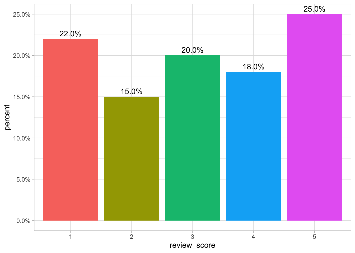

Figure 1: A bar chart of review scores

Next, we can use the date column we created earlier to determine how review scores have changed over time. First, we average the review score over each month and then plot this date using geom_smooth to make the visualisation more appealing.

We can see from the graph that review scores seem to increase slightly before dipping towards the end of 2020. After this, the scores appear to increase by an entire star on average before it begins to plateau off suggesting the scores may have start to stabilise at around 3.75 stars on average.

reviews_data %>%
  group_by(year, month)%>%
  summarise(
    review_score = mean(review_score)
  )%>%
  mutate(
    date = make_date(month = month, year = year)
  ) %>%
  arrange(date) %>%
  ggplot(aes(date, review_score)) +
  geom_smooth(se = FALSE) +
  scale_x_date(date_breaks = "1 month") +
  scale_y_continuous(limits = c(2, 4))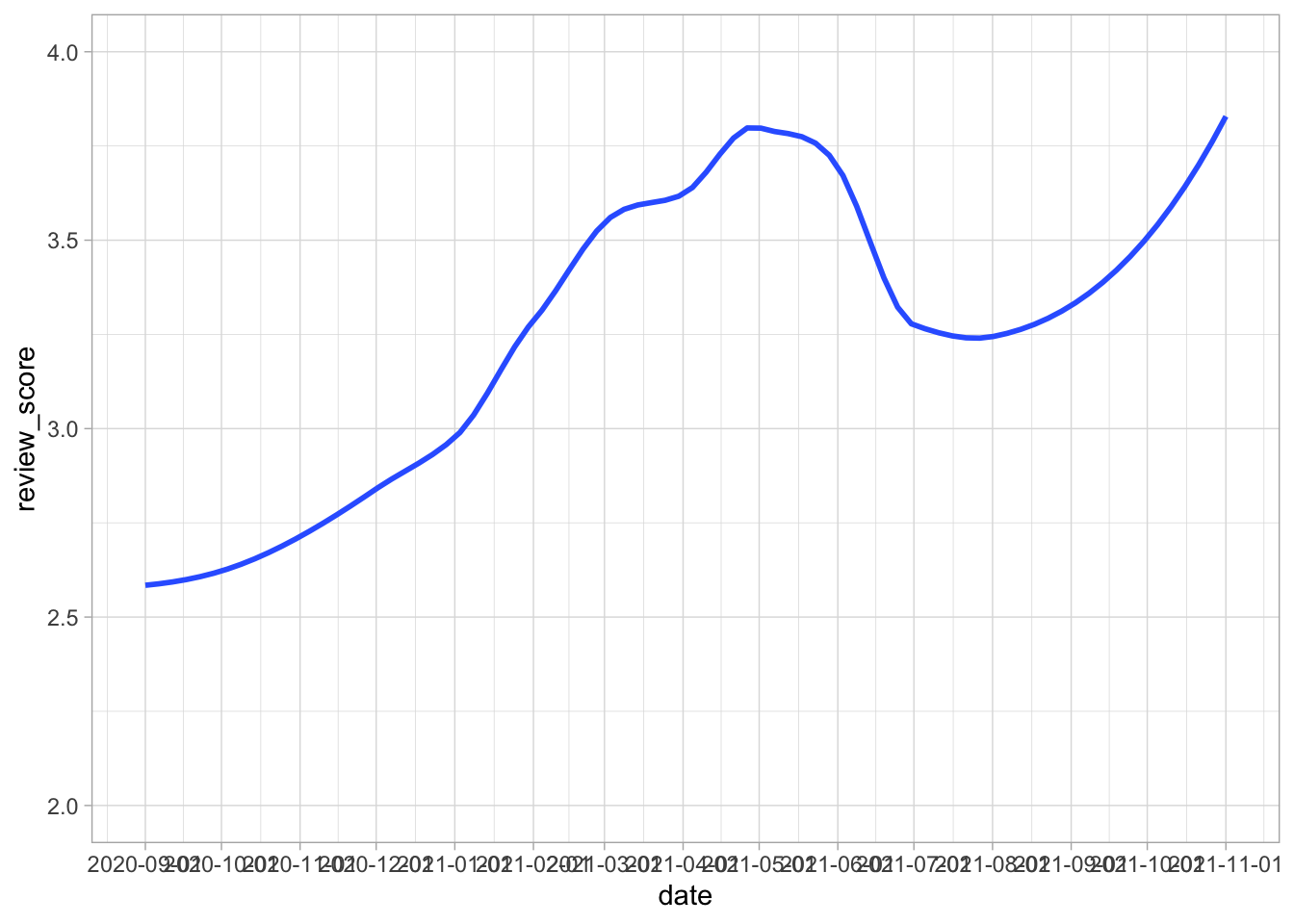

Figure 2: How review score changes over time

In our data, all the reviews came from the United Kingdom so plotting the review scores across different countries is not neccessary however for other products this visualisation may have value.

Now we have explored the review scores, we can begin to dig into the richer data source available from these reviews - the review text itself.

Text mining Amazon reviews

The two main sources of text from Amazon reviews is the review title and the body of the text itself. These two sources could be analysed separately but for this analysis, as we are only interested in the words used, we will combine both columns together.

reviews_data <- reviews_data %>%
  mutate(
    text = paste(review_title, review_text, sep = ". ")
  )

Now we have all our text data in one column, we can tidy this text so it can be more easily analysed. To do this, we will use the tidy text package. We will start by converting all the text to lower case, then extract only the words (inessence removing the whitespace and punctuation) using the unnest_token function from tidy text. Then, we remove stop words. These are words that while important for understanding, are not helpful for analysising the content of the text as they are extremely common. We do this using the anti_join function from dplyr which returns all the rows (words) in our current dataframe which match any of the words included in the stop_words dataframe. Finally, we count the number of times each word appears in our dataframe. You can see the top 10 words in the dataframe below.

data(stop_words)
review_text <- reviews_data %>%
  select(text) %>%
  mutate(
    text = str_to_lower(text)
  ) %>%
  unnest_tokens(word, text) %>%
  anti_join(stop_words) %>%
  count(word, sort = TRUE)

head(review_text, 10)

## # A tibble: 10 x 2
##    word       n
##    <chr>  <int>
##  1 watch    198
##  2 fitbit   156
##  3 versa    113
##  4 3         81
##  5 app       65
##  6 phone     62
##  7 music     61
##  8 button    51
##  9 screen    47
## 10 2         46

We can create visualisations from this data to make it easier to interpret. From this information, we can see that the words watch, fitbit and versa appear most commonly. This is not entirely surprising given the product that is being reviewed. We could remove these words from future analysis if we wanted to but for now we will leave them in place.

review_text %>%
  head(10) %>%
  mutate(
    word = reorder(word, n)
  ) %>%
  ggplot(aes(word, n)) +
  geom_col() +
  coord_flip() +
  labs(y = "Word count", x = NULL)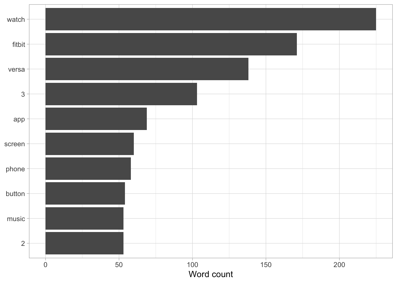

Figure 3: Most common words used within the reviews

Whilst this visualisation is informative, we could make a more appealing, and informative visualisation, called a word cloud. To do this we will use the wordcloud package. Into this function we put the column that contains the words extracted within the reviews and the number of times the words appear as well as the minimum number of times the word needs to appear to be included within the visualisation.

wordcloud(review_text$word, freq = review_text$n, min.freq = 5)

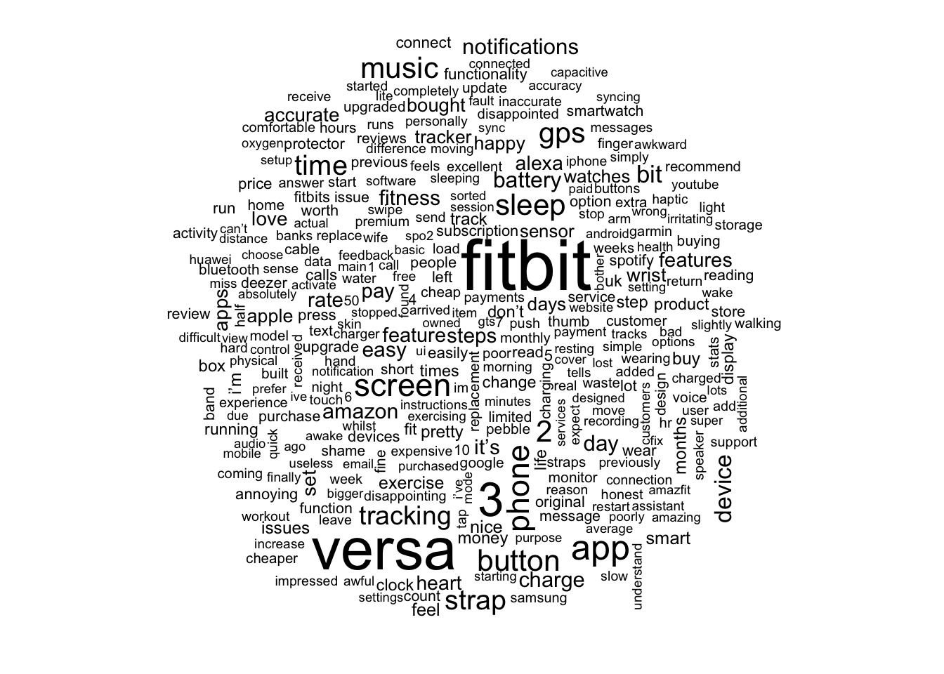
Figure 4: A wordcloud of the words most frequently used within Amazon reviews

From this visualisation, we can see much of the pattern that we saw before. However, we can also see that words such as heart, accuracy, music and battery all appear in relatively large font. While we do not know the context these words are used in, we can intimate the meaning of many of these words. For example, we know users are forming opinions on the accuracy of the wearable device. However, we do not know what metric this is in relation to or whether the accuracy is deemed to be good or poor. These are questions we could look to answer in further analysis.

Sentiment analysis

Now we have extracted the most common words, we can explore the meaning of these words. To do this we will use sentiment analysis on each word we have extracted from the reviews. To calculate the overall sentiment of the reviews we will use a sentiment lexicon. This is a list of words with an associated value based on their meaning. We will use the AFINN dictionary which assigns each word a value between -5 and 5 based on whether the word is negative or positive respectively.

To create a dataset with the sentiments included within it, we will reuse some code from above but use the inner_join function to join the afinn lexicon dictionary to our list of words. Before this, we will use the get_sentiments command to create the lexicon dictionary as an R object.

afinn <- get_sentiments("afinn")
sent_data <- reviews_data %>%
  select(text, review_score) %>%
  mutate(
    text = str_to_lower(text)
  ) %>%
  unnest_tokens(word, text) %>%
  anti_join(stop_words) %>%
  inner_join(afinn) 

sent_data %>%
  head(10)

## # A tibble: 10 x 3
##    review_score word        value
##           <dbl> <chr>       <dbl>
##  1            3 smart           1
##  2            3 smart           1
##  3            3 falling        -1
##  4            3 recommend       2
##  5            3 limited        -1
##  6            3 pretty          1
##  7            3 comfortable     2
##  8            3 pretty          1
##  9            3 stable          2
## 10            3 fine            2

Now we have our dataframe, we can visualise this data. To do this, we first group the data by word and sum the sentiment value. This means if a word is used in multiple times in the reviews the sentiment value reflects this. We then visualise this data using a bar plot and add a horixontal line to reflect the average sentiment value of the reviews.

sent_data %>%
  group_by(word) %>%
  summarise(value = sum(value)) %>%
  ggplot(aes(x = reorder(word, value),  y = value)) +
  geom_col() +
  scale_x_discrete(labels = NULL, breaks = NULL) +
  ylim(c(-5, 5)) +
  labs(x = NULL) +
  theme(legend.position = 'none') +
  geom_hline(aes(yintercept = mean(value), color = "red"))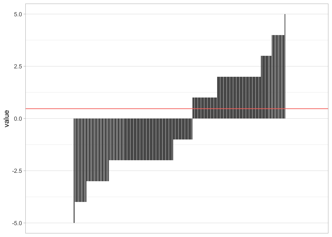 

Figure 5: The sentiment of each word present within the reviews

The graph above shows the average sentiment of the words used in the review is positive with a value of 0.2427056. We can also see that there are a limited number of uses of very positive or very negative words with most words scoring either 2 or -2.

Now we have looked at sentiment across the entire dataset, lets look at it based on the review score. First, we will create a dataframe with the mean sentiment value from the words used in each review score. Then we will create the same plot as above, but add a facet wrap by review_score to create 5 separate plots for each review score. We will then add a line to reflect the average in each plot using the dataframe we created earlier.

mean <- sent_data %>%
  group_by(review_score) %>%
  summarise(
    average = mean(value)
  )

sent_data %>%
  group_by(word) %>%
  summarise(value = sum(value),
            review_score = review_score) %>%
  ggplot(aes(x = reorder(word, value), y = value, fill = review_score)) +
  geom_col() +
  scale_x_discrete(labels = NULL, breaks = NULL) +
  ylim(c(-5, 5)) +
  labs(x = NULL) +
  theme(legend.position = 'none') +
  facet_wrap(~review_score) +
  geom_hline(data = mean, aes(yintercept = average), color = "red")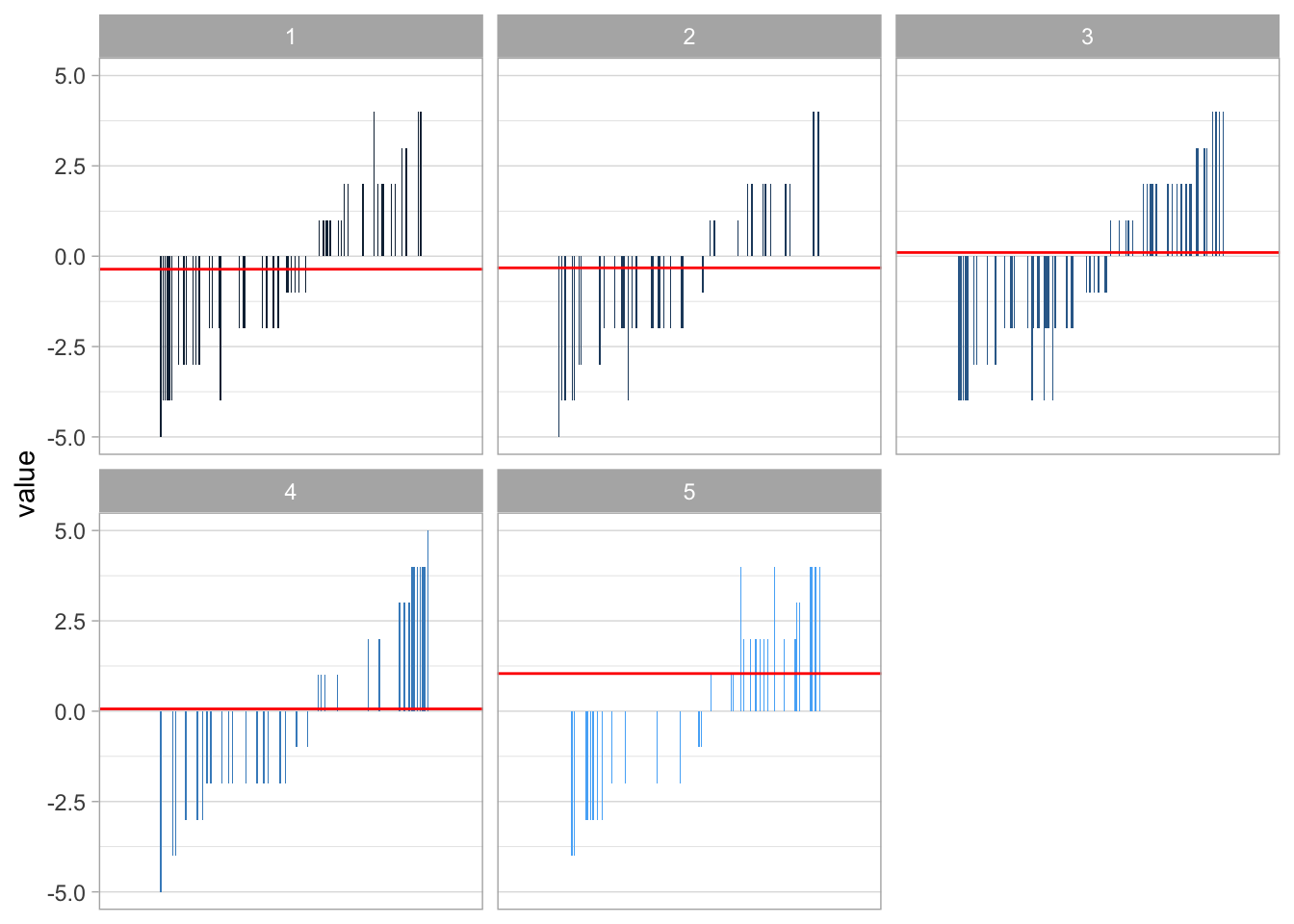

Figure 6: Visualising the sentiment value across reviews with different scores

From this visualisation, we can see that the average sentiment increases as the review score increases. We can also see that as the review score increases less negative words are used while more positive words are used. However, even five star reviews contain some negative words. Whilst this is to be expected, it is interesting to see that we can potentially distinguish review score based on the words used in the review text. To further this analysis, we could look to build a machine learning algorithm to predict the review score based on the words used within the review.

Conclusion

In the above analysis, we used web scraping to extract data from Amazon reviews. We then analysed begun by analysing the review score and then analysed the text included in the review by looking at word frequency followed by performing sentiment analysis. This analysis could be further extended by using machine learning methodologies or by other forms of text analysis such as tf-idf or topic modelling.