
Introduction to Tidy Models
TL;DR
TidyModels is a framework for creating a wide range of models in R. Today, we will look to construct models using the TidyModels framework to determine which factors impact the price of cars. Then, we will fit models and use these to predict the price of cars to determine how well our factors can describe the price of cars. Finally, I will give my thoughts on the framework and why it will be my go to for all modeling in R going forwards.
Introduction
I already have a couple of posts on machine learning on this blog. However, all these post utilise the now out-dated caret package in R. R Studio has more recently released the TidyModels series of packages (the modeling equivalent t the TidyVerse). In this post we will utilise the TidyModels framework to consturct a number of models, explore these models and then use these models to predict an outcome. At the end, I will briefly discuss my thoughts on the TidyModels framework.
We will use a dataset from Kaggle which can be found at: https://www.kaggle.com/hellbuoy/car-price-prediction. There is a problem statement include with this dataset that we will attempt to address today. In summary, a company is looking to create a new car that will sell for a high price in the American car market. They want to know two main things: which variables significantly predict the price of cars and how well do these variables describe the price of cars. To answer this question, we will create a number of models to explore the variables that contribute to the price of cars and secondly we will create a machine learning model to ascertain how well these variables predict the price of cars.
Getting started …
Before we start, let’s library in the packages we will use. The main ones will be the tidyverse and tidymodels series of packages.
library(tidyverse)
library(tidymodels)
library(kableExtra)
library(rpart.plot)
library(vip)
set.seed(1234)
Summarising our data
theme_set(theme_light())
car_prices <- read.csv("/Users/jonahthomas/R_projects/academic_blog/content/english/post/2021-09-27-introduction-to-tidy-models/CarPrice_Assignment.csv")
kable(head(car_prices))| car_ID | symboling | CarName | fueltype | aspiration | doornumber | carbody | drivewheel | enginelocation | wheelbase | carlength | carwidth | carheight | curbweight | enginetype | cylindernumber | enginesize | fuelsystem | boreratio | stroke | compressionratio | horsepower | peakrpm | citympg | highwaympg | price |
|---|---|---|---|---|---|---|---|---|---|---|---|---|---|---|---|---|---|---|---|---|---|---|---|---|---|
| 1 | 3 | alfa-romero giulia | gas | std | two | convertible | rwd | front | 88.6 | 168.8 | 64.1 | 48.8 | 2548 | dohc | four | 130 | mpfi | 3.47 | 2.68 | 9.0 | 111 | 5000 | 21 | 27 | 13495 |
| 2 | 3 | alfa-romero stelvio | gas | std | two | convertible | rwd | front | 88.6 | 168.8 | 64.1 | 48.8 | 2548 | dohc | four | 130 | mpfi | 3.47 | 2.68 | 9.0 | 111 | 5000 | 21 | 27 | 16500 |
| 3 | 1 | alfa-romero Quadrifoglio | gas | std | two | hatchback | rwd | front | 94.5 | 171.2 | 65.5 | 52.4 | 2823 | ohcv | six | 152 | mpfi | 2.68 | 3.47 | 9.0 | 154 | 5000 | 19 | 26 | 16500 |
| 4 | 2 | audi 100 ls | gas | std | four | sedan | fwd | front | 99.8 | 176.6 | 66.2 | 54.3 | 2337 | ohc | four | 109 | mpfi | 3.19 | 3.40 | 10.0 | 102 | 5500 | 24 | 30 | 13950 |
| 5 | 2 | audi 100ls | gas | std | four | sedan | 4wd | front | 99.4 | 176.6 | 66.4 | 54.3 | 2824 | ohc | five | 136 | mpfi | 3.19 | 3.40 | 8.0 | 115 | 5500 | 18 | 22 | 17450 |
| 6 | 2 | audi fox | gas | std | two | sedan | fwd | front | 99.8 | 177.3 | 66.3 | 53.1 | 2507 | ohc | five | 136 | mpfi | 3.19 | 3.40 | 8.5 | 110 | 5500 | 19 | 25 | 15250 |
tidymodels_prefer()Within our dataset, we have the variable price which we will use as the outcome variable for our models. We then have the car_ID and carName column which can be used as identification leaving 23 variables we can use as exploratory variables in our models. Let’s examine a few of these variables to begin our analysis, let’s start with price.
car_prices %>%
  summarise(
    mean = mean(price, na.rm = TRUE),
    std = sd(price, na.rm = TRUE),
    min = min(price, na.rm = TRUE),
    max = max(price, na.rm = TRUE)
  )
## mean std min max
## 1 13276.71 7988.852 5118 45400Now lets look at the distribution of the price variable. To do this we will create a hisotgram.
ggplot(car_prices, aes(x = price)) +
  geom_histogram(binwidth = 2500)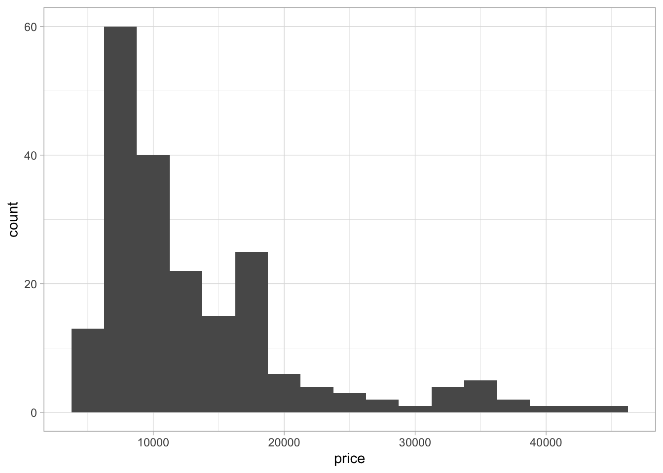
We can see in this histogram that our data is not normally distributed. The data has a left skew and also is looking like it might be slightly bi-modal as there are two peaks in the data. A larger initial peak at around $10000 and a second significantly smaller peak at around $35000. Due to the size of the second peak, it is worth noting but not a hugely significant finding especially due to the relatively small size of the dataframe.
Next, we will look at the correlation between the numeric variables in our dataset. Highly correlated variables can be problematic in some models so this step gives us an idea whether we should be concerned about this and which variables we should give extra consideration to. To do this, we will use the corrplot package.
library(corrplot)
corr <- cor(car_prices %>% select(where(is.numeric)))
corrplot(corr, method = "square", type = "lower")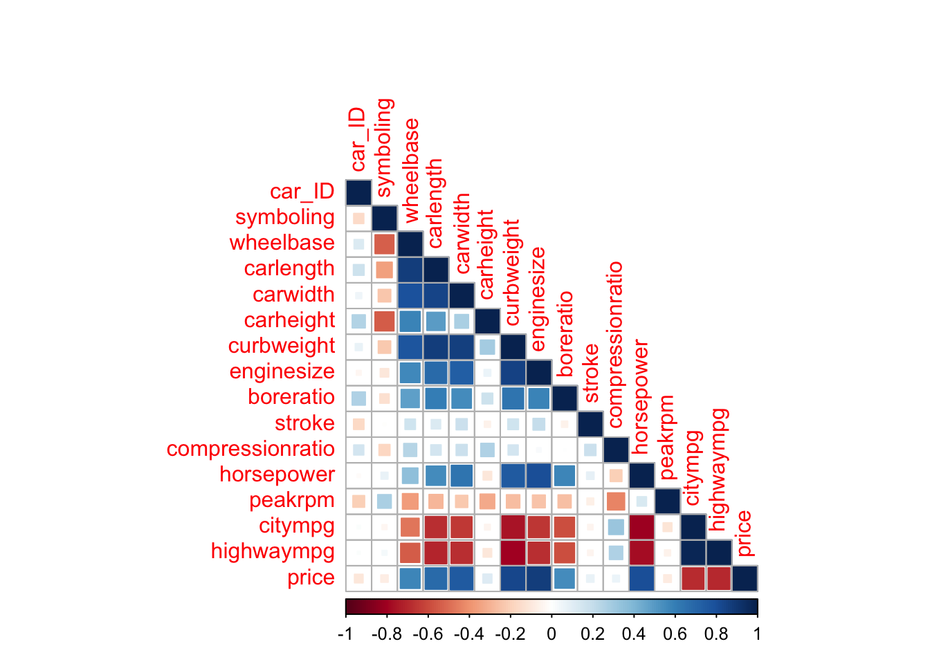
Now we have some understanding of our data, we can start building our models. We will start by creating a linear model.
Creating a linear model
When creating models using the tidymodels framework. We start by creating a model specification. To do this we will use a model function (in this case linear_reg()) and then we set the engine we want the model to use (in this case lm). Secondly, we will create a work flow for the model. To do this, we will use the work flow function, followed by adding a model into that work flow using the add_model function. Work flows in tidymodels bundle together the pre-processing, modelling and post processing steps. They also provide a convenient series of steps that are consistent across a wide range of models.
Netx, we will add some pre-procesing to our workflow. We will use recipes to do this. Recipes are a method to combine all the pre-processing steps, as well as provide the formula for the model. For this analysis, we will model car price as the response variable and use all other variables in the dataset (denoted by .) as exploratory variables. We will then use the step_dummy function to convert all nominal variables in our dataframe to dummy variables. We will then use the step_corr function to remove any predictors that have a correlation greater than ± 0.9. We will then add this recipe to our linear model work flow.
Now we have our work flow complete with pre-processing and model specification, we can use it to fit our model. We use the fit function and provide it with the work flow and the dataset we want the work flow to be applied to. We can then use the extract_fit_parsnip function to retrieve the model fit. Using the tidy function from the broom package provides this information in a clean and easy to understand format.
For this analysis, we will use the vip function (from the package vip) to plot a graph of the variables with the most importance. These are the variables that have the largest influence on car price and therefore help us to answer our key question.
Creating a linear model
Lets begin creating our linear model by setting the model specification. For this model, we will use the “lm” engine. Then, we will create a work flow and add the model specification to it.
linear_model <- linear_reg() %>% set_engine("lm")
linear_wflow <- workflow() %>% add_model(linear_model)
Next, we will create the recipe for our model. To do this, we will start by setting the formula for our model. Then, for the linear model, we need to convert all our nominal predictors to dummy variables an then we will remove any highly correlated variables. Then, we will add this recipe to our work flow.
linear_recipe <- recipe(price ~ ., data = car_prices %>% select(-car_ID, -CarName)) %>%
  step_dummy(all_nominal_predictors()) %>%
  step_corr(all_predictors(), threshold = 0.9)

linear_wflow <- linear_wflow %>% add_recipe(linear_recipe)
Next, we will fit the model by providing the workflow and the relevant data to the fit function.
linear_fit <- fit(linear_wflow, car_prices %>% select(-car_ID, -CarName))We can then examine our model parameters by extracting them from our fitted model and then tidying this data.
linear_fit %>% extract_fit_parsnip() %>% tidy()## # A tibble: 39 × 5
## term estimate std.error statistic p.value
## <chr> <dbl> <dbl> <dbl> <dbl>
## 1 (Intercept) -31809. 14755. -2.16 0.0325
## 2 symboling 12.6 230. 0.0545 0.957
## 3 wheelbase 37.2 94.5 0.394 0.694
## 4 carlength -64.6 49.0 -1.32 0.189
## 5 carwidth 642. 238. 2.69 0.00780
## 6 carheight 49.3 123. 0.401 0.689
## 7 curbweight 3.39 1.69 2.01 0.0464
## 8 enginesize 126. 25.5 4.94 0.00000190
## 9 boreratio -1863. 1562. -1.19 0.235
## 10 stroke -4489. 882. -5.09 0.000000973
## # … with 29 more rowsFinally, we can extract the importance of the variables within the model using the vip package’s vip function. This gives us our model summary, including the intercept, the beta value (estimate) for each variable, the standard error, the t statistic and the p value.
linear_fit %>% extract_fit_parsnip() %>% vip()
Looking at the graph above, we see that stroke is the most important variable in determining price, followed by engine size and then the type of engine. This tells us that these variables are likely to have the largest impact on the price of cars.
Price difference by brand
In the graph above, we can see that we removed the car ID and car name column. We did this as these columns will almost certainly predict price, however it has little value to a company. However, the car name column contains information regarding the brand that produced each car. Once again, this might not seem massively useful (our company cannot stick a BMW badge on it’s car to increase the value) however it it interesting to understand if price differs by brand. To explore this, we can plot the data on a bar chart.
car_prices %>%
  separate(CarName, into = c("brand", NA)) %>%
  group_by(brand) %>%
  summarise(
    mean = mean(price),
    sem = sd(price)/sqrt(length(price)),
    upper = mean + sem,
    lower = mean - sem,
    n = n()
  ) %>%
  ggplot(aes(reorder(brand, mean), mean)) +
  geom_col() +
  geom_errorbar(aes(ymax = upper, ymin = lower)) +
  coord_flip() +
  xlab("Car brand") +
ylab("Mean price ($)") 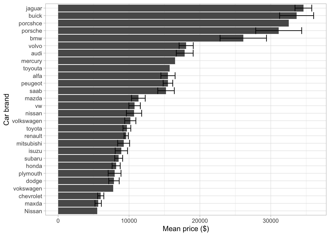
We can see from this, that certain car brands (such as Jaguar and Porsche) have a significantly higher price for their cars than other brands such as Honda or Mazda. This tells us that different car brands do have different prices however these differences are likely to be caused by other differences in the car, no simply the brand name. Therefore, we will not use brand in future models however it could be included to answer a different research question.
Creating a multi-adaptive regression spline (MARS) model
Whilst the linear model above i useful and tells us some of the key variables that best model price, one model will never give us all the answers. Therefore, we will create two more models using our data and we can then assess the variable importance across all three models to hopefully get a more comprehensive idea of our data. Next, we will use a multi-adaptive regression spline model.
mars_recipe <- recipe(price ~ ., data = car_prices %>% select(-car_ID, -CarName)) %>%
  step_dummy(all_nominal_predictors()) %>%
  step_corr(all_numeric_predictors()) %>%
  step_scale(all_numeric_predictors()) %>%
  step_center(all_numeric_predictors())

mars_spec <- mars() %>% set_engine("earth") %>%  set_mode("regression")
mars_wflow <- workflow() %>% add_model(mars_spec)
mars_wflow <- mars_wflow %>% add_recipe(mars_recipe)
mars_fit <- fit(mars_wflow, car_prices %>% select(-car_ID, -CarName))
mars_fit %>%
  extract_fit_engine() %>%
  vip()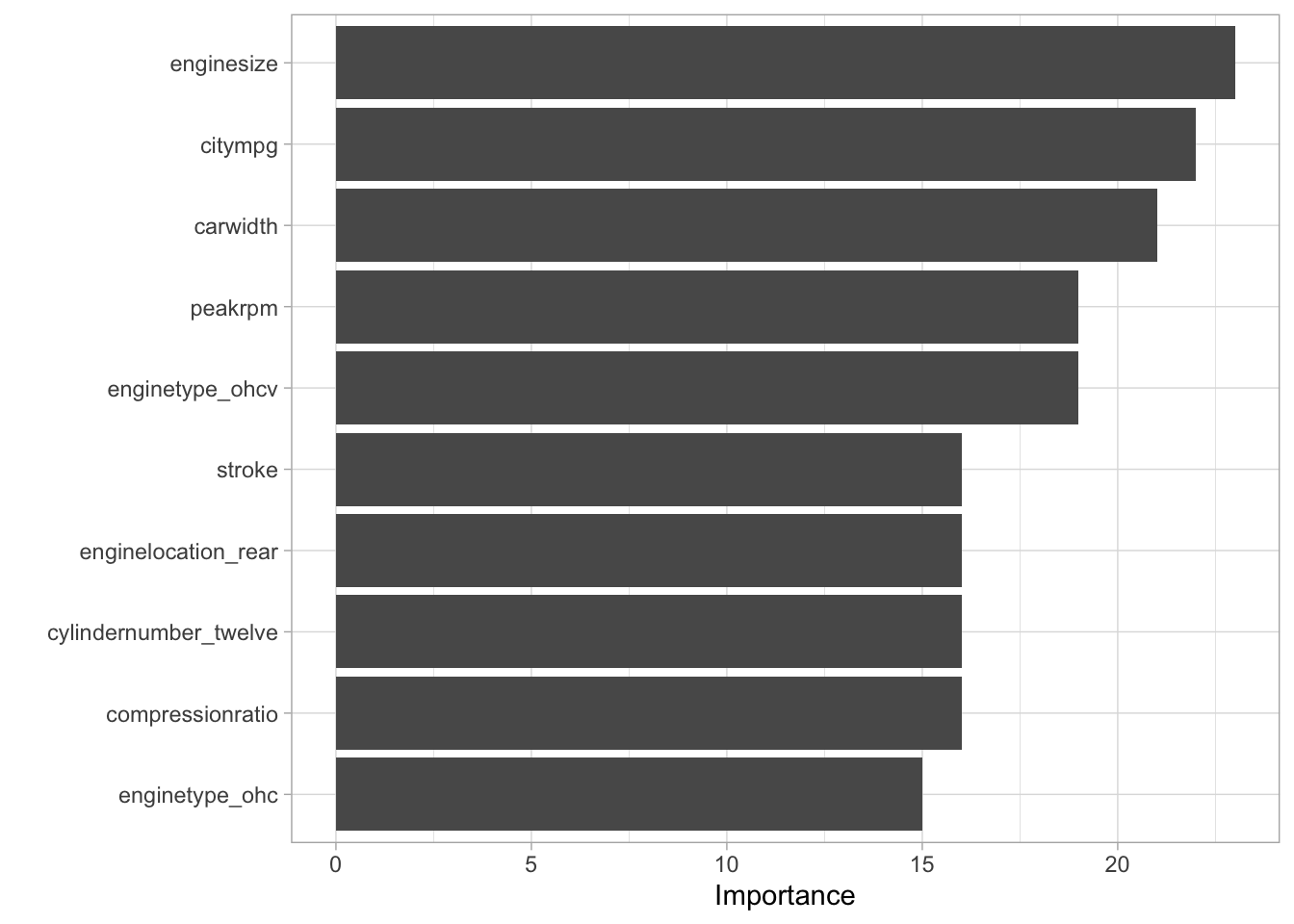
We can see from this graph, engine size appears to have the largest importance followed by city mpg and car width. We can see this differs from the variables that had the highest importance from the linear model highlighting that different modeling approaches can lead to additional insight. To enhance this point, lets look at a decision tree model.
Creating a decision tree model
dt_recipe <- recipe(price ~ ., data = car_prices %>% select(-car_ID, -CarName)) %>%
  step_dummy(all_nominal_predictors()) %>%
  step_corr(all_numeric_predictors())

dt_spec <- decision_tree() %>% set_engine("rpart") %>% set_mode("regression")

dt_wflow <- workflow() %>% add_model(dt_spec) %>% add_recipe(dt_recipe)

dt_fit <- fit(dt_wflow, car_prices %>% select(-car_ID, -CarName))

rpart.plot(dt_fit$fit$fit$fit)
dt_fit %>%
  extract_fit_parsnip() %>%
  vip()
We can see once again, the variables and the order of these variables differ from the other models. However, we can begin to see some variables that are frequently scoring well across all the models.
Creating a machine learning model
Now we understand which variables are likely to have the largest impact on our data, we can use these variables to create a predictive model that will predict the value of cars. To do this, we will start by splitting our dataset into a training and testing set. This will allow us to ascertain how accurately our model (and the variables within it) describe the price of cars.
First, we need to split our data into a training and testing set.
price_split <- initial_split(car_prices, prop = 0.8, strata = price)
price_train <- training(price_split)
price_test <- testing(price_split)
This framework from TidyModels gives a very simple method to split the data. We start by setting the split and providing the data we want to split, as well as the proportion of data to place in the train set (80% in our case). We can also set a variable to stratify the split by. This means we can ensure that both our training and testing datasets are representative of of data. This is particularly useful when our data is skewed. In our case, we have a large left skew so by stratifying the sample we can counter this issue.
Now, let’s use a linear model, and then a decision tree.
linear_spec <- linear_reg() %>% set_engine("lm")
linear_wflow <- workflow() %>% add_model(linear_spec)
linear_recipe <- recipe(price ~ enginesize + stroke + citympg + carwidth + enginetype, data = price_train) %>%
  step_dummy(all_nominal_predictors()) %>%
  step_corr(all_numeric_predictors(), threshold = 0.9)
linear_wflow <- linear_wflow %>% add_recipe(linear_recipe)
linear_fit <- fit(linear_wflow, price_train)
linear_predict <- predict(linear_fit, price_test)
price_test_results <- bind_cols(linear_predict, price_test %>% select(price))
ggplot(price_test_results, aes(price, .pred)) +
  geom_point() +
  geom_abline(lty = 2) +
  coord_obs_pred()
metrics <- metric_set(rmse, rsq, mae)
metrics(price_test_results, truth = price, estimate = .pred)
## # A tibble: 3 × 3
## .metric .estimator .estimate
## <chr> <chr> <dbl>
## 1 rmse standard 3529.
## 2 rsq standard 0.836
## 3 mae standard 2593.The above metrics give us an idea of how well our model, and the variables within it, describe the price of cars. We can see from the R squared that our variables explain 88.6% of the variance in car price. This highlights that our variables do a very good job of describing the differences in car price. The RMSE (root mean squared error) and MAE (mean absolute error) show how far our predictions were from the true value. We can see we are currently off by a few thousand dollars. Let’s see if we can improve that with a decision tree model.
We will create a decision tree using our training data as before, but we will also tune the hyper-parameters of the model to explore whether we can achieve better performance.
First, we set a specification for the model and include the parameters we want to tune in the model function. In this case, we will tune the cost complexity and tree depth variables.
tune_spec <-
  decision_tree(
    cost_complexity = tune(),
    tree_depth = tune()
  ) %>%
  set_engine("rpart") %>%
  set_mode("regression")
We can then set the grid we want to tune over. This function selects a number of ‘sensible’ values. In our case, we ask for five values of each parameter creating a grid of 5x5 (25) possible decision trees.
tree_grid <- grid_regular(cost_complexity(),
                          tree_depth(),
                          levels = 5)
We then need to create some data to perform our cross-validation on. We will use the vfold_cv to do this.
folds <- vfold_cv(price_train %>% select(-car_ID, -CarName))We then create our workflow
dt_tune_recipe <- recipe(price ~ enginesize + stroke + citympg + carwidth + enginetype, data = price_train) %>%
  step_dummy(all_nominal_predictors()) %>%
  step_corr(all_numeric_predictors())

tree_wf <- workflow() %>%
  add_model(tune_spec) %>%
  add_recipe(dt_tune_recipe)
We then fit our model by providing the workflwo and then using the tune grid function. We set the resamples to the folds we create earlier and the grid (the options to tune over) to the grid we created above.
tree_res <-
  tree_wf %>%
  tune_grid(
    resamples = folds,
    grid = tree_grid
    )
We can then use the select best function to select the best tree from the tuning we performed above. We can then use this tree in the finalize work flow function to create our final decision tree model.
best_tree <- tree_res %>%
  select_best()

final_wf <-
  tree_wf %>%
  finalize_workflow(best_tree)
Finally, we can use the last fit function with our final work flow to apply our model to the test data and get our predicted values. We can then use the metric system as we did above with the linear model and extract our RMSE, R squared and MAE.
final_fit <- final_wf %>%
  last_fit(price_split)

metrics(final_fit %>% collect_predictions(), truth = price, estimate = .pred)
## # A tibble: 3 × 3
## .metric .estimator .estimate
## <chr> <chr> <dbl>
## 1 rmse standard 3113.
## 2 rsq standard 0.886
## 3 mae standard 2168.final_fit %>%
extract_fit_engine() %>%
rpart.plot(roundint = FALSE)
We can see by using a different model and tuning the hyper-parameters we have improved our R squared value to 90.5%. We can also see that our MAE has decreased to just over $2000 whilst our RMSE has increased slightly. This shows our predictors are describing the price of cars well and that by using different models we can produce improvements in performance.
My thoughts on the TidyModels Framework
To put it simply, I think the framework is excellent for anyone that is looking to use models in data analysis or machine learning. The main benefit in my opinion, is the consistency in code between all the models we can create. If you can write a linear model, you can write a KNN model, or a decision tree with a few simple changes. This make the code significantly easier and understand the decisions an individual has made as it remains consistent rather than changing with each model. Secondly, the number of useful helper functions makes performing previously tedious tasks much more simple. For example, splitting data and creating dummy variables can now be performed in a few lines of codes rather than entire data manipulation pipelines.
It did take me a little while to get TidyModels to run successfully, mainly due to a large number of outdated packages I had loaded! However, once these were updated everything appeared to run smoothly and the addition of helper functions such as tidymodels_prefer and tidymodels_update should limit these problems as much as possible.