
Introduction to Python Data Analysis
Introduction to Python
Before we begin running any analysis, lets import a few libraries that will be useful during our analysis. We will import pandas and numpy to conduct our data manipulation and analysis and the matplotlib library for visualisations.
import pandas as pd
import numpy as np
import matplotlib as plt
import seaborn as sns
from IPython.core.interactiveshell import InteractiveShell
InteractiveShell.ast_node_interactivity = 'all'
To begin the analysis we will load our dataset using the read_csv function from the pandas library. We can then use the head function to preview our data.
data = pd.read_csv("/Users/jonahthomas/R_projects/academic_blog/content/english/post/2021-09-06-introduction-to-data-analysis-in-python/basic_income_dataset_dalia.csv")
data.head()
| country_code | uuid | age | gender | rural | dem_education_level | dem_full_time_job | dem_has_children | question_bbi_2016wave4_basicincome_awareness | question_bbi_2016wave4_basicincome_vote | question_bbi_2016wave4_basicincome_effect | question_bbi_2016wave4_basicincome_argumentsfor | question_bbi_2016wave4_basicincome_argumentsagainst | age_group | weight |
|---|---|---|---|---|---|---|---|---|---|---|---|---|---|---|
| AT | f6e7ee00-deac-0133-4de8-0a81e8b09a82 | 61 | male | rural | no | no | no | I know something about it | I would not vote | None of the above | None of the above | None of the above | 40_65 | 1.105.534.474 |
| AT | 54f0f1c0-dda1-0133-a559-0a81e8b09a82 | 57 | male | urban | high | yes | yes | I understand it fully | I would probably vote for it | A basic income would not affect my work choices | It increases appreciation for household work a… | It might encourage people to stop working | 40_65 | 1.533.248.826 |
| AT | 83127080-da3d-0133-c74f-0a81e8b09a82 | 32 | male | urban | NaN | no | no | I have heard just a little about it | I would not vote | ‰Û_ gain additional skills | It creates more equality of opportunity | Foreigners might come to my country and take a… | 26_39 | 0.9775919155 |
| AT | 15626d40-db13-0133-ea5c-0a81e8b09a82 | 45 | male | rural | high | yes | yes | I have heard just a little about it | I would probably vote for it | ‰Û_ work less | It reduces anxiety about financing basic needs | None of the above | 40_65 | 1.105.534.474 |
| AT | 24954a70-db98-0133-4a64-0a81e8b09a82 | 41 | female | urban | high | yes | yes | I have heard just a little about it | I would probably vote for it | None of the above | It reduces anxiety about financing basic needs | It is impossible to finance | It might encoura… | 40_65 |
Now we have loaded the data, we can explore some of the variables. For the purpose of demonstration, we will look at age (a numeric variable), gender, rural and dem_full_time_job (categorical variables) using the describe function.
data['age'].describe()
data['gender'].describe()
data['rural'].describe()
data['dem_full_time_job'].describe()
count    9649.000000
mean       37.712716
std        12.270630
min        14.000000
25%        28.000000
50%        40.000000
75%        46.000000
max        65.000000
Name: age, dtype: float64


count     9649
unique       2
top       male
freq      5094
Name: gender, dtype: object


count      9649
unique        2
top       urban
freq       6878
Name: rural, dtype: object


count     9649
unique       2
top        yes
freq      5702
Name: dem_full_time_job, dtype: object
As we can see above the describe function gives a summary of each variable whether it is numeric or categoric. We can see that there is a total of 9649 responses to the questionnaire with an average respondent age of 37.7 years. 5094 respondents were male, 6878 lived in an urban area and 5702 were in full time employment. Whilst this information is useful to give us a basic understanding of our data, we may also be interested in looking at whether gender has an affect on whether a respondent is employed full time.
data.groupby('gender').agg({'dem_full_time_job': 'count'})
| dem_full_time_job |
|---|
| 4555 |
| 5094 |
We can see more men and in full time employment than women. We could group by multiple variables if we wanted to see how they both affected another variable(s).
data.groupby(['gender', 'rural']).agg({'dem_full_time_job': 'count'})
| dem_full_time_job | ||
|---|---|---|
| gender | rural | |
| female | rural | 1410 |
| urban | 3145 | |
| male | rural | 1361 |
| urban | 3733 |
We can see from this summary that the employment rate between males and females in rural areas are very similar (with more women employed than men) however the differences in urban areas are more stark with 600 more men in full time employment than women. It is worth noting, these findings are in no way causitive, they are simply an exploration to show potentially interesting trends.
Basic Data Visualisation
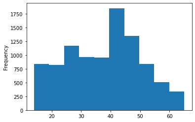
data['age'].plot.hist(bins = 10)
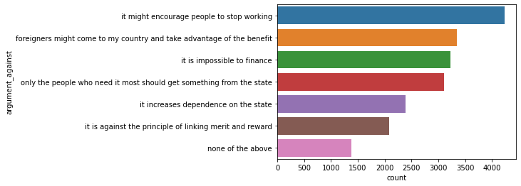
vote_against = pd.DataFrame(data['question_bbi_2016wave4_basicincome_argumentsagainst'].str.split('|').explode())
vote_against['question_bbi_2016wave4_basicincome_argumentsagainst'] = vote_against['question_bbi_2016wave4_basicincome_argumentsagainst'].str.lower()
vote_against['question_bbi_2016wave4_basicincome_argumentsagainst'] = vote_against['question_bbi_2016wave4_basicincome_argumentsagainst'].str.strip()
vote_against = vote_against.groupby('question_bbi_2016wave4_basicincome_argumentsagainst').agg(count=('question_bbi_2016wave4_basicincome_argumentsagainst', 'count')).sort_values('count', ascending = False)
vote_against.index.name = 'argument_against'
vote_against.reset_index(inplace=True)
ax = sns.barplot(x = "count", y = "argument_against", data = vote_against)
sns.catplot(x = 'age', y = 'question_bbi_2016wave4_basicincome_vote', kind = 'box', data = data)
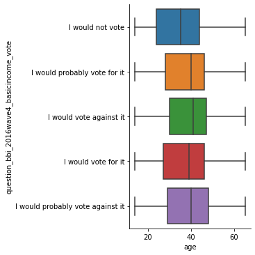
This boxplot highlights one key factor in our data; those who say they would not vote tend to be younger than those that say they would vote. It seems that amongst those that said they would vote, the direction of this vote is not highly dependent upon age.
Would the vote pass?
data['vote'] = data['question_bbi_2016wave4_basicincome_vote'].str.contains("for")
vote = data.groupby('vote').agg(count = ('vote', 'count'))
vote.index.name = 'vote'
vote.reset_index(inplace=True)
sns.barplot(x = 'vote', y = 'count', data = vote)
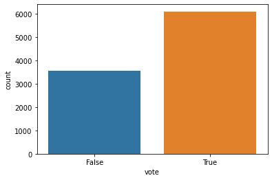
From the graph above, we can say that it is likely the vote would pass! To calculate this, we used a simplistic approach. First, we create a column called vote that is set to true if the respondent says they either would vote for basic income or are likely to vote for basic income. All other values are set to false. The graph clearly shows the majority of individuals would vote for a basic income suggesting the vote would pass.
we could also now look at this voting status by age group and see the differences.
vote_age = data.groupby(['vote', 'age_group']).agg(count = ('vote', 'count'))
vote_age.index.name = 'vote'
vote_age.reset_index(inplace=True)
sns.barplot(x = 'age_group', y = 'count', hue = 'vote', data = vote_age)
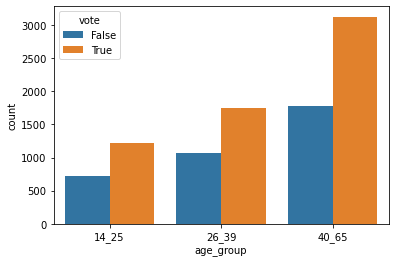
The most notable pattern from this graph is the majority of respondents come from the 40-65 year old category. It also suggests that individuals in this category may slightly more likely to vote for a basic income than younger individuals (shown by the greater height difference between the bars).
Now we have looked at voting status by age, we can also look at voting status by whether the respondent has children.
vote_child = data.groupby(['vote', 'dem_has_children']).agg(count = ('vote', 'count'))
vote_child.index.name = 'vote'
vote_child.reset_index(inplace=True)
sns.barplot(x = 'dem_has_children', y = 'count', hue = 'vote', data = vote_child)
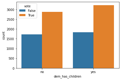
We can see from this that having children seems to make people slightly more likely to vote for a basic income than not. Again, this is not a causitive relationship, just an exploration of the datasets.
A basic model
Python has a number of libraries that allow us to build models to represent our data. The following is by no means an in depth look at any of these libraries, merely an initial look at some basic linear models. I hope to create a more comprehensive post on modelling in Python in the near future.
Today, we will use Python’s Patsy library to create a linear model. We will start with a very simple model looking to explain the way an individual votes based on their age.
from sklearn.linear_model import LinearRegression

vote = np.array(data['vote']).reshape(-1,1)
age = np.array(data['age']).reshape(-1,1)

model = LinearRegression()
model.fit(vote, age)

print('Intercept:', model.intercept_)
print('Coefficient:', model.coef_)
print('R squared:', model.score(vote, age))
LinearRegression()


Intercept: [37.57560427]
Coefficient: [[0.21720479]]
R squared: 7.294238969335343e-05
Lets talk through this one line at a time. First, we import the linear regression model from the scikit learn library. Next, we take the vote and age columns from our dataframe and reshape them each into a single column. Then, we create a linear regression model before using the fit function to fit the model to the vote and age data.
We can then examine the model intercept and coefficient which we print as the output. Finally, we can examine the R squared value. In this model, we can see that age explains a very very samll amount of the variation in voting pattern. Therefore, further analysis would need to look at other variables to explain the trends in voting pattern.
Conclusions
Above we have walked through a very basic data analysis in Python. We start by creating some summary data, before creating some visualisations of our data and finally creating a basic linear model. Whilst this analysis is by no means extensive, I hope it highlights how a simple dataset could be explored using Python. In future, I hope to perform some more complex analyses in Python including experimenting with machine learning models.